This project explores machine learning techniques to classify wine quality as “good” or “bad” based on physicochemical properties. Two models, K-Nearest Neighbors (KNN) and Logistic Regression (LR), were used, evaluated, and optimized. The aim was to compare performance metrics like accuracy, F1-score, precision, and recall, and find the optimal model.

🎯 Objective
The objective of this project is to build and evaluate machine learning models that can accurately predict wine quality (good or bad) based on chemical features such as acidity, sugar content, pH, and alcohol levels.
# Best model parameters based on previous results:IDW
best_penalty = 'l1'
best_C = 10.0
best_solver = 'liblinear'

# Re-train the model on full training data
lr = LogisticRegression(penalty=best_penalty, C=best_C, solver=best_solver, max_iter=1000)
lr.fit(train_data, train_labels)

# Make predictions on test data
test_pred = lr.predict(test_data)
from sklearn.model_selection import train_test_split
# Split data
X = df_final.drop(columns=['quality'])
y = df_final['quality']
X_train, X_test, y_train, y_test = train_test_split(X, y, test_size=0.2, random_state=42)
from sklearn.model_selection import train_test_split
# Split data
X = df_final.drop(columns=['quality'])
y = df_final['quality']
X_train, X_test, y_train, y_test = train_test_split(X, y, test_size=0.2, random_state=42)
📂 Code Structure
1. Data Loading and Preprocessing
The dataset used is from the UCI repository. It includes 4,898 rows of white wine data and 12 columns (features). The target variable, `quality`, is binarized into “good” (quality > 5) and “bad” (quality <= 5).
import pandas as pd
# Load dataset
df = pd.read_csv('winequality-white.csv', delimiter=';')
# Binarize target variable
df['quality'] = df['quality'].apply(lambda x: 1 if x > 5 else 0)
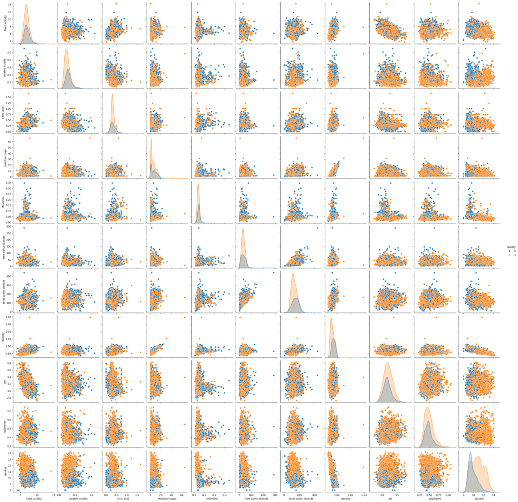
To identify redundant features, correlations, and visualize relationships between the features and the target, we created pair plots.
import seaborn as sns
sns.pairplot(df, hue = 'quality') # I want to compare all files with quality
plt.show()

3. Feature Engineering and Selection
We dropped features with high correlation (above 0.8) and unnecessary ones. After examining the pair plot and correlation matrix, density was dropped due to its strong correlation with residual sugar.
# Dropping highly correlated features
df_final = df.drop(columns=['density'])
from sklearn.model_selection import train_test_split
# Split data
X = df_final.drop(columns=['quality'])
y = df_final['quality']
X_train, X_test, y_train, y_test = train_test_split(X, y, test_size=0.2, random_state=42)
# Best model parameters based on previous results: KNN
best_k = 11
best_distance = 'manhattan'
best_weights = 'distance'
# Re-train the model on full training data
knn = KNeighborsClassifier(n_neighbors=best_k, weights=best_weights, metric=best_distance)
knn.fit(train_data, train_labels)
5-2. Logistic Regression (LR):
- Regularized LR tested with L1 and L2 penalties, and values of
C(regularization strength). - The best LR model used L1 regularization with
C=10.
# Best model parameters based on previous results:IDW
best_penalty = 'l1'
best_C = 10.0
best_solver = 'liblinear'

# Re-train the model on full training data
lr = LogisticRegression(penalty=best_penalty, C=best_C, solver=best_solver, max_iter=1000)
lr.fit(train_data, train_labels)

# Make predictions on test data
test_pred = lr.predict(test_data)
6. Model Evaluation
The models were evaluated using accuracy, F1-score, precision, recall, and ROC-AUC.
from sklearn.metrics import roc_auc_score
# Calculate the AUC score
auc_score = roc_auc_score(test_labels, knn_probs)

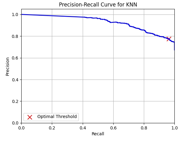
from sklearn.metrics import precision_recall_curve

# Calculate precision and recall values
precision, recall, thresholds = precision_recall_curve(test_labels, knn_probs)

# Plot the precision-recall curve
plt.figure()
plt.plot(recall, precision, color='b', lw=2)
plt.xlabel('Recall')
plt.ylabel('Precision')
plt.title('Precision-Recall Curve for KNN')
plt.xlim([0.0, 1.0])
plt.ylim([0.0, 1.05])
plt.grid(True)

# Calculate F1 scores at each threshold
f1_scores = [2 * (p * r) / (p + r) if (p + r) > 0 else 0 for p, r in zip(precision, recall)]

# Determine the optimal threshold that maximizes the F1 score
optimal_threshold = thresholds[np.argmax(f1_scores)]

# Mark the optimal threshold on the precision-recall curve
plt.scatter(recall[np.argmax(f1_scores)], precision[np.argmax(f1_scores)], c='r', marker='x', s=100, label='Optimal Threshold')
plt.legend(loc="lower left")

# Print the optimal threshold
print("Optimal Threshold:", optimal_threshold)

plt.show()

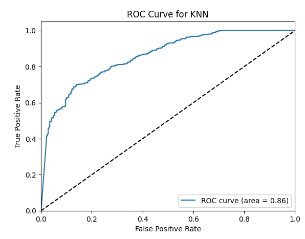
7. ROC Curve and Optimal Threshold for KNN
We generated the ROC curve for the KNN model and determined the optimal threshold for F1 score maximization
from sklearn.metrics import roc_curve, auc

# ROC Curve for KNN
fpr, tpr, thresholds = roc_curve(y_test, knn_probs)
roc_auc = auc(fpr, tpr)
optimal_threshold = thresholds[np.argmax([f1_score(y_test, [1 if x >= t else 0 for x in knn_probs]) for t in thresholds])]

Optimal Threshold for KNN: 0.3090528018168291
F1 Score using Optimal Threshold: 0.8592692828146145
🧠 Results
The KNN model using Manhattan distance and inverse distance weighting (IDW) provided the best results with an F1 score of 0.87, outperforming Logistic Regression.
Conclusion
KNN with k=11 and Manhattan distance outperformed logistic regression for this task. However, logistic regression performed competitively and may be preferred when model interpretability or faster predictions are necessary.
⚙️ Skills & Tools
- Languages/Tools: Python, Pandas, NumPy, Scikit-learn
- Data Visualization: Matplotlib, Seaborn
- Model Evaluation: Precision-recall analysis, ROC-AUC curves, cross-validation