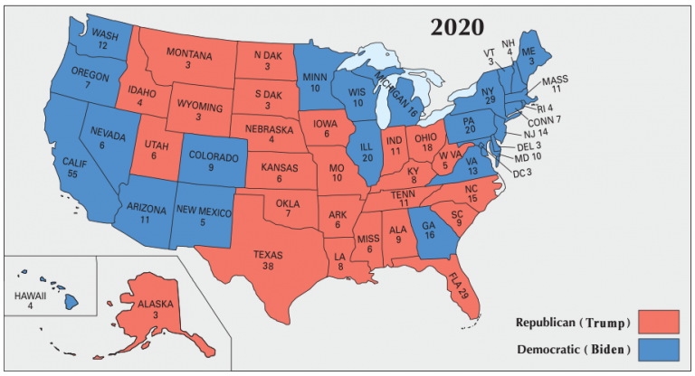
This project investigates voter behavior using income data from Washington State, employing machine learning to predict voting patterns. The model integrates geographical and income data, improving voter prediction models using batch processing. Collaborating with team members focusing on gender, education, and age-based studies in other states, this project aims to inform policymakers by providing insights into complex electoral dynamics.
base_map = census_blocks.plot(column='relative_error', legend=True, figsize=(12, 8))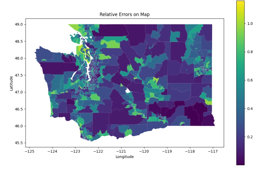
- Extracts and filters income data categorized by income levels from Washington State’s census tracts, prepping it for machine learning analysis.
- Implements a basic neural network model (SimpleNN) with income data to predict voting outcomes using preprocessing and normalization techniques.
# Training loop
for epoch in range(500):
    optimizer.zero_grad()
    outputs = model(X_train)
    loss = criterion(outputs, y_train)
    loss.backward()
    optimizer.step()
    if epoch % 10 == 0:
        print(f'Epoch [{epoch+1}/500], Loss: {loss.item()}')
plt.plot(losses[10:], label='Training Loss') #The code plots only the data points for the training loss after excluding the first 10 epochs.
plt.xlabel('Epoch')
plt.ylabel('Loss')
plt.legend()
plt.show()

# Evaluation
y_pred = model(X_test).detach().numpy()
rmse = np.sqrt(mean_squared_error(y_test.numpy(), y_pred))
print(f'RMSE: {rmse}')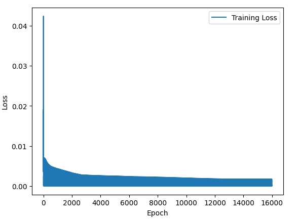
- Compares models like Linear Regression, Polynomial Regression, Random Forest, and SVR. The Random Forest model delivered the best performance with an RMSE of 0.0797.
This enhanced deep neural network incorporates batch normalization and dropout layers to prevent overfitting while capturing complex relationships between income and voting patterns. Various optimizers, such as ADAM and ADAGRAD, were tested to enhance model performance.
optimizer2 = optim.Adam(model.parameters(), lr=0.001) #New: SGD ->> ADAM
#optimizer = torch.optim.SGD(model.parameters(), lr=0.001) : Original
#optimizer = optim.Nadam(model.parameters(), lr=0.001)
#optimizer = optim.RMSprop(model.parameters(), lr=0.001)

import torch
num_epochs = 500
losses = []
for epoch in range(num_epochs):
    for i,(train_X, train_y)  in enumerate(county_dataloader):
      epoch_loss = 0.0
      if i<32:

        # Convert lists to PyTorch tensors
        features = torch.tensor(train_X)
        target = torch.tensor(train_y)

        # Forward pass, loss computation, and backward pass
        outputs = model(features)
        # print(outputs) # issue here
        loss = custom_loss(outputs, target)
        optimizer2.zero_grad()
        loss.backward()
        optimizer2.step()
        epoch_loss += loss.item()
        average_epoch_loss = epoch_loss /50
       # losses.append(loss.item())
        losses.append(average_epoch_loss)
    if epoch % 10 == 0:
print(f'Epoch [{epoch+1}/{num_epochs}], Loss: {loss.item()}')🧪 Methodology Overview
Geospatial and income data were collected from the U.S. Census and voting records from Washington State. GIS techniques (centroid mapping) were used to match electoral precincts with census tracts. After extensive data cleaning and standardization, the final dataset incorporated income levels and election results across various precincts.
import geopandas as gpd # 1. Importing Data and Libraries
import pandas as pd

# Filter precincts with overlap_percentage >= 50
filtered_precincts = overlap_precincts[overlap_precincts['overlap_percentage'] >= 50]

# Now, filtered_precincts contains only the precincts with overlap_percentage >= 50
# Visualize the selected census block and precincts that are approximating it
census_blocks.loc[[CENSUS_BLOCK_INDEX]].explore('STATEFP')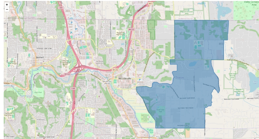
# Visualize the filtered precincts with their Biden proportion
filtered_precincts.explore('Biden_proportion')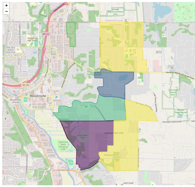
# Show the approximation error
base = census_blocks.loc[[CENSUS_BLOCK_INDEX]].plot('STATEFP', color='red', alpha=0.5)
filtered_precincts.plot('STATEFP', color='yellow', ax=base, alpha=0.5)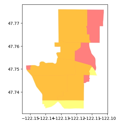
Model Development and Testing
- Linear Regression & Polynomial Regression: Simple models as a baseline.
from sklearn.linear_model import LinearRegression # LInear Regression
linear_model = LinearRegression()
linear_model.fit(X_train_np, y_train_np)- Random Forest: Best performance, capturing nonlinear relationships in voting patterns.
from sklearn.ensemble import RandomForestRegressor # Random Forest Regressor
random_forest_model = RandomForestRegressor(n_estimators=100, random_state=42)
random_forest_model.fit(X_train_np, y_train_np)- SVR (Support Vector Regression): Moderate performance, capturing nonlinearity.
from sklearn.svm import SVR # Support Vector Regressor(SVR)
svr_model = SVR(kernel='rbf')
svr_model.fit(X_train_np, y_train_np)- Simple Deep Learning (DeepNN): Incorporates advanced layers to prevent overfitting and capture intricate patterns in data.
import torch.nn as nn
import torch.optim as optim
# Define SimpleNN class
class SimpleNN(nn.Module):
    def __init__(self):
        super(SimpleNN, self).__init__()
        self.fc1 = nn.Linear(20, 32)
        self.fc2 = nn.Linear(32, 1)
        self.relu = nn.ReLU()

    def forward(self, x):
        x = self.relu(self.fc1(x))
        x = self.fc2(x)
        return x

# Initialize model, loss, and optimizer
simple_model = SimpleNN()
criterion = nn.MSELoss()
optimizer = optim.SGD(simple_model.parameters(), lr=0.001)- Improved Deep Learning (DeepNN)
# Define DeepNN class with BatchNorm and Dropout
class DeepNN(nn.Module):
    def __init__(self):
        super(DeepNN, self).__init__()
        self.fc1 = nn.Linear(20, 32)
        self.bn1 = nn.BatchNorm1d(32)
        self.fc2 = nn.Linear(32, 64)
        self.bn2 = nn.BatchNorm1d(64)
        self.fc3 = nn.Linear(64, 64)
        self.bn3 = nn.BatchNorm1d(64)
        self.fc4 = nn.Linear(64, 1)
        self.relu = nn.ReLU()
        self.dropout = nn.Dropout(0.5)

    def forward(self, x):
        x = self.relu(self.bn1(self.fc1(x)))
        x = self.relu(self.bn2(self.fc2(x)))
        x = self.dropout(x)
        x = self.relu(self.bn3(self.fc3(x)))
        x = self.fc4(x)
        return x
# Initialize improved deep learning model
deep_model = DeepNN()for i, (val_X, val_y) in enumerate(county_dataloader2):
if i >= 32:
start_time = time.time()
features = torch.tensor(val_X)
target = torch.tensor(val_y)
model.train()
outputs = model(features)
# Loss
loss = custom_loss(outputs, target)
losses1.append(loss.item()) # Store loss in losses1
# RMSE, MAE, R^2
actuals = target.cpu().numpy() # Actual
predictions = outputs.detach().cpu().numpy() # Prediction
rmse_scores.append(np.sqrt(mean_squared_error(actuals, predictions)))
mae_scores.append(mean_absolute_error(actuals, predictions))
r2_scores.append(r2_score(actuals, predictions))
# Optimizer backing and Zero
optimizer.zero_grad()
loss.backward()
optimizer.step()
# Recoding the time
end_time = time.time()
timestamps1.append(end_time - start_time) # Store time in timestamps1
num_batches += 1
# Evaluation
print("Average RMSE:", np.mean(rmse_scores))
print("Average MAE:", np.mean(mae_scores))
print("Average R^2:", np.mean(r2_scores))Results
- The Random Forest model provided the best accuracy with the lowest RMSE of 0.0797, followed by SVR and Polynomial Regression. The study demonstrates that integrating income and geospatial data through machine learning leads to effective voting behavior predictions.
Challenges
- GIS Integration: Aligning different datasets from NY and WA required significant GIS manipulation.
- Overfitting: Initial deep learning models with many layers suffered from overfitting, prompting model simplification.
- Income Binning: Grouping income data into larger intervals improved interpretability without compromising on the granularity.
The Random Forest model was most effective in predicting voter behaviors based on income. This framework can be extended by incorporating more demographic variables (e.g., education, age) and applying it to other states to yield broader insights into electoral patterns.
- U.S. Census Bureau
- Harvard University Database
- GIS Resources
